
Abstract
BACKGROUND AND PURPOSE: Researchers and clinical radiology practices are increasingly faced with the task of selecting the most accurate artificial intelligence tools from an ever-expanding range. In this study, we sought to test the utility of ensemble learning for determining the best combination from 70 models trained to identify intracranial hemorrhage. Furthermore, we investigated whether ensemble deployment is preferred to use of the single best model. It was hypothesized that any individual model in the ensemble would be outperformed by the ensemble.
MATERIALS AND METHODS: In this retrospective study, de-identified clinical head CT scans from 134 patients were included. Every section was annotated with “no-intracranial hemorrhage” or “intracranial hemorrhage,” and 70 convolutional neural networks were used for their identification. Four ensemble learning methods were researched, and their accuracies as well as receiver operating characteristic curves and the corresponding areas under the curve were compared with those of individual convolutional neural networks. The areas under the curve were compared for a statistical difference using a generalized U-statistic.
RESULTS: The individual convolutional neural networks had an average test accuracy of 67.8% (range, 59.4%–76.0%). Three ensemble learning methods outperformed this average test accuracy, but only one achieved an accuracy above the 95th percentile of the individual convolutional neural network accuracy distribution. Only 1 ensemble learning method achieved a similar area under the curve as the single best convolutional neural network (Δarea under the curve = 0.03; 95% CI, −0.01−0.06; P = .17).
CONCLUSIONS: None of the ensemble learning methods outperformed the accuracy of the single best convolutional neural network, at least in the context of intracranial hemorrhage detection.
ABBREVIATIONS:
- AUC
- area under the curve
- CNN
- convolutional neural network
- ICH
- intracranial hemorrhage
- SVM
- support vector machine
As clinical support systems in radiology evolve, artificial intelligence has become prevalent for supporting myriad operations ranging from order entry, computer-aided diagnosis, clinical decision support, triage, to back-end analytics. With the development of new tools for design, implementation, and deployment of artificial intelligence–based systems, many in-house support tools are more accessible to clinicians as well as researchers.1 In fact, many radiology practices are continuously developing and deploying their internal artificial intelligence tools and support systems, and the use of these tools has increased exponentially.
At the same time, researchers and clinical radiology practices are increasingly faced with the task of selecting the most accurate tools from an ever-expanding range. With multiple methods available for the same task, combining the results of multiple tools presents an intriguing possibility. Such “crowd-sourcing” may be able to achieve better performance than any individual method. At the same time, there is the risk of corrupting the results of better-performing methods with those from weaker ones.
For example, while multiple artificial intelligence methods for segmentation of intracranial hemorrhage (ICH) have been very successful,2,3 those for identification and progression of ICH can have variable accuracy.4,5 Part of this variability derives from differences in the characteristics of the data used for training and the population encountered in practice. It is tempting to use the best-performing method, but best performance on one specific data set does not necessarily guarantee best performance on another.
Ensemble learning may mitigate this high variability by pooling multiple methods. Since its introduction >2 decades ago,6,7 ensemble learning has garnered substantial attention as a tool for improving the performance, accuracy, and robustness of existing medical image-interpretation methods.8 It relies on a meta-algorithmic technique wherein multiple machine learning methods are trained individually and aggregated together. This approach has been successfully applied to multiple medical problems, including identification of lung cancer cells,9 colon polyp detection,10 automated classification of pulmonary bronchovascular anatomy in CT scans,11 and the differential diagnosis of focal liver lesions detected on CT scans.12
In this study, we sought to test the utility of ensemble learning for determining the best combination of models from a set of 70 models that were individually trained to identify ICH (in all intracranial compartments). Furthermore, we investigated whether ensemble deployment is preferred over the use of the single best model. We tested the hypothesis that an ensemble of different models, developed using a single training set, will outperform each individual model in the ensemble.
MATERIALS AND METHODS
Data
We used a retrospective data set of de-identified clinical head CT scans from 134 unique patients treated at the Massachusetts General Hospital (institutional review board protocol 2015P000607). Written consent was not required by the institutional review board, given the retrospective use of existing clinically available data. The clinical images were acquired under standard clinical protocols in our tertiary care hospital from January 2015 to September 2018. Patients were excluded if external hardware was visible in the scan. Images were obtained (Somatom Force; Siemens) with an exposure time of 1000 ms and a section thickness of 1 mm. Each section in the axial plane in the CT data set was annotated by the treating neuroradiologists, not part of this study, as “no-ICH” or “ICH” (Fig 1), and annotations were verified by a neuroradiologist with 20 years of experience (R.G.). Images were then down-sampled to 128 × 128 pixels. The intensity of each image was clipped between −15 and 155 HU13 and rescaled to [0, 1] for normalization. Consequently, slices were saved as TIFF images for further processing. Visible head support was removed from the images to prevent any bias due to extraneous input and to constrain the variability introduced by the head holder. Slices from the upper part and bottom of the scan FOV were excluded if they contained no or very limited parts of the head. These slices were either completely black or were at the very top of the head. The final data set included 4287 slices of which 34.4% were labeled as containing ICH.

Head CT scan slices annotated as ICH (upper and middle, arrows) and annotated as no-ICH (bottom).
The data set was split into 4 sets. Data sets 1 (48%) and 2 (12%) were used, respectively, as training and validation sets for the individual convolutional neural networks (CNNs). Data set 3 (28%) was used as a training set for the ensemble learning methods. All the remaining slices (data set 4; 12%, test set) were used to independently test the accuracy of individual CNNs as well as that of ensemble learning methods to evaluate the final performance. These steps are described in detail below.
All subsets were created at the patient level (as opposed to individual section level) to avoid superfluous correlation between images that belong to the same patient. Models were trained and their performance was evaluated on the section level, while grouping slices within each patient before partitioning to avoid bias due to overrepresentation of slices from a single patient. This partitioning resulted in 61 cases and 2034 slices in data set 1, 16 cases and 516 slices in data set 2, 38 cases and 1208 slices in data set 3, and 17 cases and 529 slices in data set 4. The slices in each set included approximately the same proportion (∼34%, varying between 32.9% and 38.8%) with ICH.
CNNs
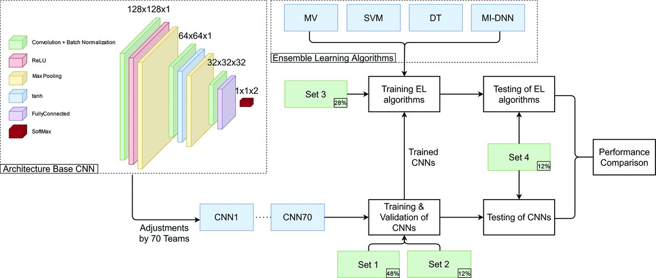
CNNs to classify slices as ICH or no-ICH were implemented by graduate students as a part of a course taught by the authors. In 2 different courses, offered between 2019 and 2021, one hundred forty students with comparable experience and education were divided into teams of 2 students each. These teams developed 70 CNNs for detecting the presence or absence of ICH in each section. Each CNN was built on the same base architecture (Fig 2), designed to provide a minimum accuracy (∼67%) and was modified, trained, and tested independently by each team on a virtual machine running on Amazon Web Services (https://aws.amazon.com/) using Matlab R2020a (MathWorks).

Flowchart of the study. The upper left corner shows the base architecture underlying all 70 CNNs, which was then structurally optimized by the 70 teams, resulting in 70 different CNNs. These were trained on data sets 1 and 2 and were used to train the 4 ensemble learning methods (MV indicates majority voting; DT, decision tree; MI-DNN, multi-input deep neural network; see text) on data set 3. Both the 70 trained CNNs and the trained ensemble methods were tested on data set 4. ReLU indicates rectified linear unit; tanh, hyperbolic tangent; EL, ensemble learning.
Each team customized the base architecture (Fig 2, left) to improve the accuracy on identical data sets. Customization included switching, adding, or removing layers and/or changing layer parameters. Parameters other than those associated with individual layers (ie, hyperparameters) were not varied so that only variations in architecture and random initialization impacted the performance during testing. Each team trained their CNN model on data set 1 for 50 epochs with a batch size of 32. They used stochastic gradient descent with a momentum optimizer with a learning rate of 0.001. Each CNN was then validated on data set 2. The final accuracy of each CNN was evaluated on data set 4 (Fig 2).
Ensemble Learning Method Training
We tested 4 different ensemble methods to explore whether the collective accuracy of 70 CNNs is higher than that of individual models. Ensemble learning methods included majority voting, decision tree, support vector machine (SVM), and the multi-input deep neural network.
In majority voting, the final prediction of the ensemble was determined to be that class predicted by the majority of CNNs. For the remaining ensemble learning methods, the probability scores for the no-ICH class were collected from each of the 70 CNNs for every image in data set 3 and were used as input. In decision tree,14 a treelike model was created in which every end branch represents a decision. One final predicted class label will be given as output. Similarly, the SVM15 also returned 1 predicted class label, and training was performed with a linear kernel. The last ensemble learning method we tested was a multi-input deep neural network. Unlike the ensemble learning methods described earlier, the multi-input deep neural network requires an additional input, namely, a CT image. The multi-input deep neural network provides a probability score for the no ICH and ICH classifications as output. A more elaborate description of these ensemble learning methods can be found in the Online Supplemental Data.
Each ensemble learning method was trained on data set 3 and tested on data set 4 (Fig 2). Test accuracy was assessed via receiver operating characteristic curves and the corresponding areas under the curve (AUCs). The code for processing of data and training of CNNs and ensemble learning methods can be found on: https://github.com/UT-RAM-AIM/Ensemble_Learning.
Statistical Analysis
By design, each CNN had a different accuracy, resulting in a normal distribution of individual accuracies across 70 individual CNNs (see Results). Thus, the accuracy of each of the 4 ensemble learning methods was compared with the distribution of individual CNNs. For this comparison, an accuracy of >95% of the individual accuracy distribution, ie, larger than 2 SDs, was considered statistically significant. We also used the minimum redundancy maximum relevance algorithm to rank the 70 CNNs in a way that optimizes the amount of information each contained. This use allowed us to determine the CNN that provides the most information to predict the correct classification while having the least amount of redundant information.16 The individual CNN with the largest relevance was ranked first, and the previous steps were repeated to determine the individual CNN with the second highest relevance and least redundancy. This process was repeated until all individual CNNs were ranked. Thus, minimum redundancy maximum relevance provided insight into the added value that each CNN contributed to the ensemble. The difference between AUCs across different ensemble methods was tested for statistical significance using a generalized U-statistic, analogous to the Mann-Whitney statistic.17
RESULTS
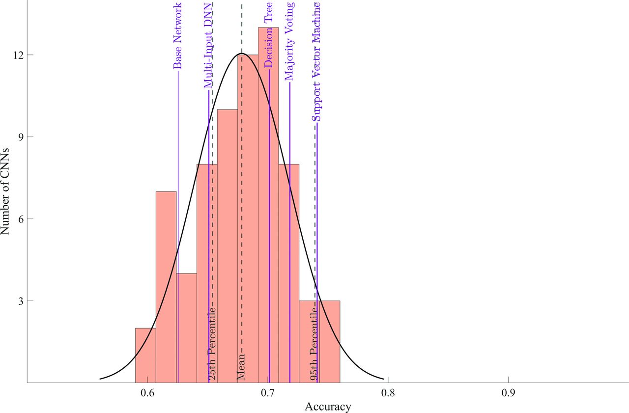
The base architecture achieved an accuracy of 62.6% on data set 4. Individual CNNs had an average test accuracy of 67.8% with a range of 59.4% to 76.0% (Fig 3).

Accuracy of individual CNNs and ensemble learning methods. The purple solid vertical lines show the accuracy achieved by each ensemble learning method, and the black dashed vertical lines show means and lower and upper 95% confidence intervals for the distribution of accuracy of individual CNNs. Additionally, the first purple solid line indicates the accuracy of the base network. DNN indicates deep neural network.
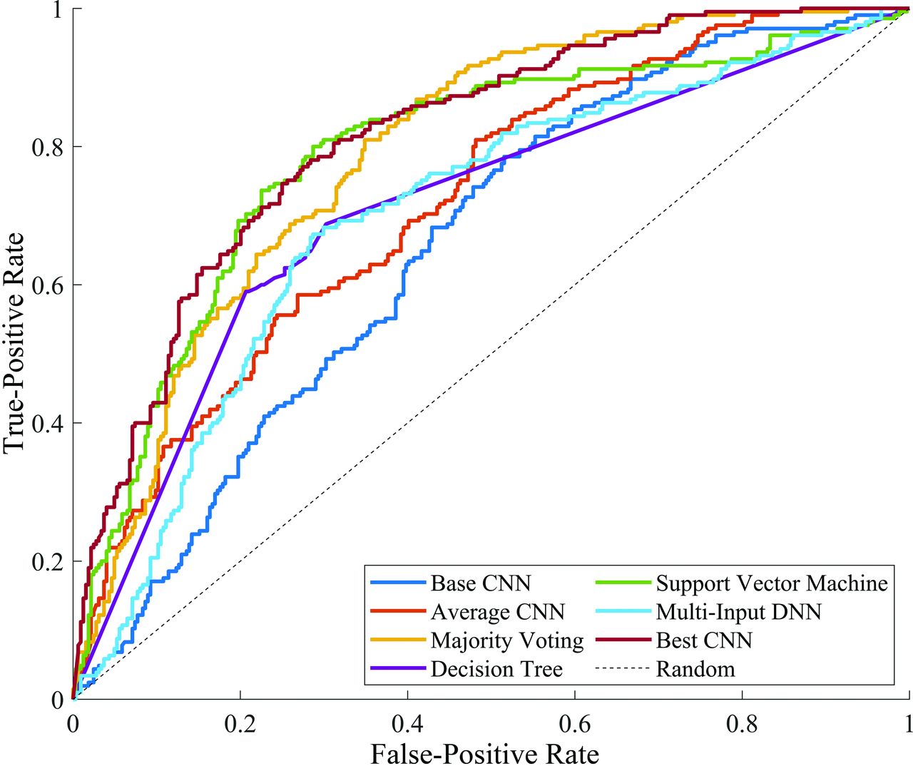
All except 1, the multi-input deep neural network, ensemble learning method outperformed the average accuracy of individual networks. However, of these, only SVM resulted in a statistically significant improvement in accuracy (ie, above the 95th percentile of the accuracy distribution from individual CNNs). None of the ensemble learning methods resulted in an accuracy greater than the individual CNN with highest accuracy (76.0%). The base architecture achieved an AUC of 0.66 (95% CI, 0.61–0.70). The AUCs attained by SVM, majority voting, and the single best CNN were, respectively, 0.79 (95% CI, 0.75–0.83), 0.79 (95% CI, 0.75–0.83), and 0.82 (95% CI, 0.78–0.85) (Fig 4).

Receiver operating characteristic curves of the base network (dark blue) and the single best CNN (dark red), the curve of the average performing CNN (orange), and ensemble learning methods. The dashed black line indicates the performance of a random classifier (ie, accuracy of 50%). DNN indicates deep neural network.
The CNN with the best accuracy had a minimum redundancy maximum relevance score of 0.15, while the second one scored only 0.0006—that is, the relevance of the single best CNN model contributed most to the ensemble learning model while the contribution of the rest was effectively zero. Additional exploration of the SVM method confirmed this observation. Training the SVM with only the network with the highest minimum redundancy maximum relevance score led to a test accuracy of 73.9%, while adding the second most relevant CNN increased the accuracy only by 0.2%–74.1%.
Statistical Analysis
The AUC for each ensemble model was statistically different from that of the base model (Fig 4; base versus decision tree, ΔAUC = 0.05; 95% CI, −0.00008−0.11; P = .05; base versus majority voting, ΔAUC = 0.14; 95% CI, 0.10−0.17; P < .001; base versus multi-input deep neural network, ΔAUC = 0.05; 95% CI, 0.0004−0.09; P = .05; and base versus SVM, ΔAUC = 0.13; 95% CI, 0.09−0.18; P < .001). The AUC for majority voting and SVM was statistically different from that of the CNN with average accuracy (average versus majority voting, ΔAUC = 0.07; 95% CI, 0.04−0.10; P < .001; and average versus SVM, ΔAUC = 0.07; 95% CI, 0.02−0.12; P = .001). All except the SVM method, including the CNN with average accuracy, were statistically different from the best-performing CNN (best CNN versus SVM, ΔAUC = 0.03; 95% CI, −0.01−0.06; P = .17). Thus, the SVM method performed better than the base model and CNN with average accuracy, but comparable with the best-performing CNN.
DISCUSSION
As mentioned earlier, many artificial intelligence–based support tools are available for a wide variety of tasks, and researching radiology practices are faced with the task of how to develop the most accurate ones for internal deployment. Ensemble learning was suggested to mitigate the high variability between multiple tools by pooling them. Our results affirm that all ensemble learning methods, with the notable exception of the multi-input deep neural network, outperform the average of different crowd-sourced CNN models. Thus, the “wisdom of crowds” can exceed the average wisdom of individuals, at least in the context of ICH identification. It was surprising that only the SVM resulted in a statistically significant improvement in accuracy. Our most important finding, however, is that none of the other methods outperformed the CNN with the highest accuracy. Thus, our study provides several important lessons for crowdsourcing.
There was a relatively large variation in accuracy of individual models, ranging from ∼0.60 to ∼0.75. However, this variability does not necessarily imply variation in information; in the context of our study, the magnitude of redundancy between the individual CNNs is high. In fact, our results show that individual models contribute little, if at all, to the overall performance of the ensemble beyond the model with the best accuracy. Uncorrelated models contribute to the ensemble most, because they can reflect features that other models do not. Consequently, a combination of different models that include different, uncorrelated features is likely to result in a better-performing ensemble.
We have adopted a “laissez-faire” approach (leaving people to take their own course, without interfering) as opposed to direct guidance. This indicates that a simple agglomeration of all models may be counterproductive and may drive the model toward the average accuracy. For example, the poorly performing models may corrupt the overall performance of the ensemble rather than collaborating to improve accuracy. In fact, it can be seen in the Results that the worst-performing single CNN achieves an accuracy (59%) lower than that of the base model (63%) accuracy. The effort of the team to improve the base architecture actually had the opposite effect in this CNN, and it most likely did not aid in improving ensemble performance. For ensemble learning over multiple individually trained models, the assumption of holistic performance from crowdsourcing may not hold, unless some basic conditions about model independence can be ensured. To that end, analysis of an ensemble of models with a feature-selection algorithm, such as minimum redundancy maximum relevance, is an essential step toward finding the optimal model.
In general but more specifically for our use case ICH identification, the apparent impact of the size of the used data set is underestimated. If the data set is not large enough, the CNNs might be unable to learn different mappings, ie, the problem does not have many solutions. Ultimately, this issue also results in redundancy within the individual CNNs. Especially in our case, ICH comprises roughly 15%18 of all cases of stroke and is, therefore, not as common in stroke. It can be difficult to acquire enough variation in a data set to allow the CNNs to learn different mappings. It may be more useful to examine safe ways of sharing data and consequently training 1 best tool with this method.
The relevant literature includes multiple studies using ensemble learning that found a positive effect from its application. For example, in their research into skin lesion classification from dermascopic images, Shahin et al19 found that by averaging the predictions of the trained ResNet-50 (accuracy 87.1%) and Inception-V3 (accuracy 89.7%) models, their accuracy improved to 89.9%. Furthermore, Rajaraman et al20 reported an accuracy increase by weighted averaging (90.97%) of their trained ResNet-18 (89.58%, highest), MobileNetV2, and DenseNet-121, to detect coronavirus disease 2019 (COVID-19) on chest radiographs. Most interesting, adding 2 more models to the ensemble in fact deteriorated the accuracy slightly. Most similar in approach to our case is the research by Zabihollahy et al,21 who trained 7 U-Nets for the localization of prostate peripheral tumors. The U-Nets differed in the depth and number of filters used in the convolution layers and were pooled using majority voting. Pooling 3 U-Nets was optimal, but this did not outperform the single best U-Net in terms of sensitivity or specificity. However, it did find the best trade-off between the two.
In contrast to the cases above, many more networks were pooled together in our study to improve the performance via ensemble learning methods. Additionally, our results did not show that an ensemble learning method outperformed the single best CNN model. However, as was also found in the research by Zabihollahy et al21 and Rajaraman et al,20 using multiple models in the ensemble learning method does not necessarily increase the performance. While Zabihollahy et al found that the overall performance did not improve when adding >3 models, in our case that point was reached at 2. Combining fewer, but structurally different, models might be more efficient as is shown in Rajaraman et al.20
CONCLUSIONS
Using ICH identification as a use case, we sought to identify the best combination from a set of 70 CNNs. Furthermore, we investigated whether an ensemble of the CNNs is preferred over using the single best CNN. It was hypothesized that an ensemble of different models, optimized from a base model, would outperform each individual CNN. While the SVM ensemble learning method did perform statistically better than the average CNN, its performance was comparable with that of the single best CNN. Even though this classroom experiment does not represent a real-world scenario when multiple artificial intelligence tools are at your disposal, it may be preferable to search for structurally different models and analyze them with a feature-selection algorithm before applying an ensemble learning method. Otherwise, a focus on the single best model may be more productive.
Footnotes
The position of E.I.S.H. is supported by a ZonMw Innovative Medical Devices Initiative (IMDI) subsidy for the B3CARE project (Dossier number: 10-10400-98-008). The funder had no role in study design, data collection and analysis, decision to publish, or preparation of the manuscript.
Disclosure forms provided by the authors are available with the full text and PDF of this article at www.ajnr.org.
References
- Received December 15, 2022.
- Accepted after revision May 7, 2023.
- © 2023 by American Journal of Neuroradiology


Jump to section
Related Articles
Cited By...
- No citing articles found.